Acoustic Doppler Current Profilers (ADCPs) are instruments used in our subsea network and other oceanographic applications to measure the currents. We collect data from two types of ADCPs, manufactured by Nortek and RDI.
An RDI ADCP before deployment showing the transducer faces where the sound beams come out as well as the pressure sensor and thermistor that senses temperature (left). At right is a Nortek current profiler prior to deployment showing the pressure and acoustic sensors (right)
These ADCPs use “sound beams” to measure water movement. Sound pulses are sent out in three or four different directions from the instrument; when sound waves strike suspended objects such as tiny particles or zooplankton, some of the energy is reflected back to the ADCP where it is detected by the instrument’s transducers. The received signal intensity gives an indication of the abundance of particles within the water. The Doppler shift of the received signal for each beam is used to determine the current velocity.
Using three separate beams, a 3D current velocity can be calculated. Some ADCPs have a fourth beam, allowing for two 3-beam calculations to be compared to gauge the reliability of the data. Also, if pings from a single beam aren't autocorrelated sufficiently (i.e. the returned echo is unreliable/ambiguous/bad/contaminated), they can be discarded and an estimate of current velocity can still be made using the other 3 beams. Some of these ADCPs also include sensors for temperature, pressure, tilt and compass heading.
Map of ADCP installations on NC as of Oct 2011.
Currently, we have 9 ADCPs in the water at a variety of locations. Some ADCPs are affixed to instrument platforms while others sit at the top of moorings (NW RCM and NE RCM) near our Endeavour site. During upcoming cruises this year we hope to install three additional ADCPs to our network.
There are some challenges, however, in using ADCPs to measure currents. There can be acoustic returns from sources other than currents detected – for example bubbles moving through the water column or fish swimming through the beams. Additionally, nearby instruments can sometimes acoustically interfere with the ADCP. Other complications include data gaps (from when the instrument was turned off or wasn’t working, for example) or changes in sampling frequency.
The data obtained from the ADCPs reveal important information about the currents at a study site, however, such data can be difficult to present in a traditional paper publication medium. Since the data represent three dimensions over long periods of time it can be challenging to flatten them out and show them in 2D. Some of data have been successfully visualized using animations but animations are difficult to represent in a printed publication.
Sample plot of north-south velocity data from the ADCP atop the Endeavour northeast regional circulation mooring. Tides are indicated by the shift from north-flowing (red) to south-flowing (blue) current.
One way to represent current data in 2D is with progressive vector diagrams like the one shown below. Progressive vector diagrams (PVDs) use a selection of depths in order to visualize the large scale, general directions of currents. Distance is not measured in this type of plot, but it is inferred from the velocity and direction of the current as well as the time interval measured. Each current vector is added onto the previous vector, starting from a central (0,0) position on a grid. This centre point represents the instrument position. Current velocity is averaged over 15 minute intervals and measured in metres per second then converted into distance (km) on the x and y axis. In essence, it is as though an individual water parcel is being followed through time along the plotted line. We can plot multiple depths on one individual PVD.
The magnitude frequency plots (small inset graphs on the progressive vector diagrams) count the number of times a particular velocity value is measured. The higher the count, the more frequently a velocity occurs, for each depth plotted. In the diagram below, very low velocities were most common at the 1907m depth, while 0.05-0.1 m/s velocities were most common at the 1827m depth. The data availability bar at the top of the plots indicates when ADCP velocity data were collected over the 3 month period represented in the diagram.
Progressive vector diagram for an ADCP on our NE RCM mooring at Endeavour between October and December 2010. This ADCP is installed at a depth of 1904m. The diagram indicates current flow in the southwest direction for the upper three depths. The lowest depth measured by the ADCP (1907m) indicates flow in the northeast direction. Inset is data availability bar (top) and a magnitude frequency plot (lower right).
Besides monitoring currents, scientists are using the ADCPs in our network for a variety of research projects examining everything from shallow shelf environments down to the deep-sea hydrothermal vents. At our Barkley and Folger locations, the West Coast Vancouver Island Coastal Marine Ecosystem (WCVI) project is studying primary (phytoplankton) and secondary (zooplankton) production in coastal marine ecosystems and the implications for fish and whales. Variability in water circulation and renewal of deep inlet waters can create variability in phytoplankton and zooplankton abundance and timing. ADCPs help scientists quantify the tidal, weekly, seasonal, and inter-annual variability of phyto- and zooplankton. Our ADCP at Folger Passage has an additional capability to study waves in this coastal zone.
Also in Barkley, the Barkley Benthic study aims to determine how disturbances affect deep sea ecosystems. Instrument platforms in Barkley Canyon are outfitted with ADCPs which will be used to monitor ecological and biological responses to episodic events.
Barkley Benthic Pod 1 during deployment, 17 May 2010. The black instrument at upper-right is a Nortek Aquadopp high-resolution current profiler.
The vertical profiler system POGO will be raised and lowered in the water column to generate profiles of the water using sensors which measure chemical, physical and biological properties. To help generate these profiles, the POGO instrument package will include a 400kHz current profiler.
Finally, the Monitoring Endeavour project uses two moorings to study the flux of heat and mass and the biogeochemical and physical processes associated with spreading ridges. Each mooring consists of numerous sensors, the uppermost one an ADCP. Two additional moorings, planned for installation this year, will allow scientists to develop special models describing deep-sea current circulations in this highly dynamic location.
The upward-looking 75 kHz ADCP goes over the edge during installation of the mooring, 13 Sept 2011.